Consumption-Based Pricing Extended

\[ \def\BB#1{{\mathbb{#1}}} \def\BF#1{{\mathbf{#1}}} \def\E{{\mathbb{E}}} \]

yedlu, Winter 2024

Consumption Pricing Characteristics

Model Assumption

One beauty of consumption-based pricing is that it requires very little assumption. One assumption that has to be satisfied is the investor is able to trade arbitrarily-small \(\xi\) units of asset.

Here’s a list of assumptions that the general consumption-based pricing do not assume:

Assumption	Notes
Complete Markets	Measures individual-level willingness to pay, everyone can have different \(p\) under incomplete markets
Specific Return Distribution	Can take any return distribution
Representative/Marginal Investor	The SDF can be heterogenous to measure different types of investors
Specific Utility Functions	Can take any form form of utility functions
Market Equilibrium	Willingness to pay do not need market equilibrium to exist
2-Period Model	Can be expanded to multi-period form (later on)
Specific Beginning Endowment	Can take any level of endowment

Reaching Equilibrium

In much rigor terms, \(p\) denotes individual investor’s willingness to pay to an asset. From above we know that the market does not have to be in eqilibrium for using the consumption-based pricing.
We will show now that, nevertheless, the market will finally be in congruent with the individual willingness to pay, reaching an equilibrium.
To begin with, purchasing \(\xi\) units of asset in extra will increase the utility in the future by (discounted to today):

\[\begin{aligned} & \beta \E [u(c_{t+1} + \xi x_{t+1}) - u(c_{t+1})] \\ = & \beta \E [u'(c_{t+1}) \, \xi x_{t+1} + ...] \end{aligned}\]

For an arbitrarily small \(\xi\), only the first-order Taylor Expansion matters.

Similarly, purchasing \(\xi\) units of asset will decrease today’s consumption. Using first-order Taylor expansion:
\[\begin{aligned} & u(c_t - \xi v_t) \\ = & u'(c_t) \xi v_t + ... \end{aligned}\]

Optimality is reached if the investor is indifferent to buy additional \(\xi\) units of asset. How does market reach equilibrium:

Scenario	Mechanism
\(v_t > p_t\)	Investor buys more asset because it is below valuation, then drives \(c_t\) down and \(\E [c_{t+1}]\) up. Convexity drives the SDF down, hence \(v_t\) dropped till equilibrium.
\(v_t < p_t\)	Investor buys less asset because it is above valuation, driving \(c_t\) up and \(\E [c_{t+1}]\) down. Convexity drives the SDF up, hence \(v_t\) increased till equilibrium.
\(v_t = p_t\)	In equilibrium.

Interconnected Random Variable

From above we know that neither \(p\) and \(c\) are exogenous. They are linked through the consumption-based pricing model and interact each other. Specifically,

• knowing \(\E [mx]\) yields the willingness to pay \(p\);
• knowing \(p\) yields investment decisions today.

Mean-Variance Frontier (Hansen-Jagannathan Bounds)

Derivation

Given an asset’s riskiness, is there a reasonable bound for the return of the asset? We will try to derive the mean-variance frontier from our consumption pricing model.

\[\begin{aligned} 1 &= \E [mR^i] \\ &= \E[m] \E[R^i] + \sigma(m, R^i) \\ &= \frac{\E[R^i]}{R^f} + \rho (m, R^i) \sigma(m) \sigma(R^i) \end{aligned}\]

Rewriting the equation we would have:
\[\begin{aligned} \E [R^i] - R^f &= - R^f \rho (m, R^i) \sigma(m) \sigma(R^i) \\ R^f = \frac{1}{\E[m]} \implies \E [R^i] - R^f &= - \rho (m, R^i) \frac{\sigma(m)}{\E[m]} \sigma(R^i) \end{aligned}\]

By Cauchy-Schwarz inequality:
\[\begin{aligned} \mid \E [R^i] - R^f \mid &\leq \frac{\sigma(m)}{\E[m]} \sigma(R^i) \end{aligned}\]

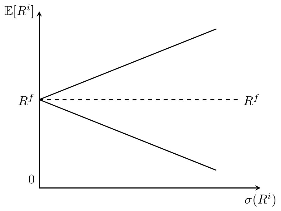
Graphical Illustration

Sample Mean-Variance Frontier

Assets on the upper bound:
\[\begin{aligned} \E [R^i] &= R^f + \frac{\sigma(m)}{\E[m]} \sigma(R^i) \end{aligned}\] implies the correlation \(\rho(m, R^i) = -1\). The asset return has perfect negative correlation with the SDF (hence perfect positive correlation with consumption). These types of asset bring higher volatility to consumption, thus investors would require a much higher excess return. One example would be stocks that goes high when market is bullist and plummets when market is bearish.

The lower bound, on the opposite,
\[\begin{aligned} \E [R^i] &= R^f - \frac{\sigma(m)}{\E[m]} \sigma(R^i) \end{aligned}\] describes assets with high returns when consumptions are low. Consider insurances: normal investors would not require a high excess return on insurance products generally, as long as they can use these products to smoothen consumption levels across time and states.

Illustration

We can compare assets within the wedge-shaped mean-variance frontier through two ways:

• Horizontally. If two assets (their corresponding points in the graph) lies under one horizontal line, then they have the same expected returns (\(\E[R^i]\)). The asset on the left has lower overall risk (\(\sigma(R^i)\)) which can be attributed to idiosyncratic risks.
  
• Vertically. If two assets (their corresponding points in the graph) lies under one vertical line, then they have the same overall risk. The one that has a higher expected return (on the top) has a higher consumption-payoff correlation.

Sharpe Ratio

The Sharpe ratio measures the excess return (per unit of risk) and is defined as:
\[\begin{aligned} \frac{\E[R^i] - R^f}{\sigma(R^i)} \end{aligned}\]

We can connect Sharpe ratio with the mean-variance frontier:
\[\begin{aligned} \mid \frac{\E[R^i] - R^f}{\sigma(R^i)} \mid &\leq \frac{\sigma(m)}{\E[m]} \end{aligned}\] Intuition: the slope of the mean-variance frontier wedge is the maximum Sharpe ratio available.

Multi-Period Pricing

Setting

Now, the asset pays a stream of cash flows \(\{\delta_{t+j}\}\) in the future. How should we price this multi-period asset?

Optimization

Let’s revisit the optimization problem:
\[\begin{aligned} \max_{c_{t+j}} & \quad \BB{E}_t \left[\sum_{j = 0}^{\infty} \beta^j u(c_{t+j})\right] \\ \text{s.t.} & \quad c_t(\xi) = e_t - p_t \xi \\ & c_{t+j}(\xi) = e_{t+j} + \delta_{t+j} \xi \quad (j \leq 1) \end{aligned}\]

Rearranging the objective function:
\[\begin{aligned} \max_{\xi} & \quad \left[u(e_t - p_t \xi) + \BB{E}_t \left[ \sum_{j = 1}^{\infty} \beta^j u(e_{t+j} + \delta_{t+j} \xi) \right] \right] \end{aligned}\]

The first-order condition (FOC) w.r.t \(\xi\) of this objective function be:
\[\begin{aligned} - p_t u'(c_t) + \E_t \left[\sum_{j = 1}^{\infty} \beta^j \delta_{t+j} u'(c_{t+j}) \right] = 0 \end{aligned}\]

Solution

Solving for the price (willingness to pay):
\[\begin{aligned} p_t &= \E_t \left[\sum_{j = 1}^{\infty} \beta^j \frac{u'(c_{t+j})}{u'(c_t)} \delta_{t+j} \right] \end{aligned}\]

We define the multi-period stochastic discount factor (SDF) as:
\[\begin{aligned} m_{t+j} &:= \beta^j \frac{u'(c_{t+j})}{u'(c_t)} \quad (j \geq 1) \end{aligned}\]

Risk-Adjusted Form

As in the two-period model, we can also rewrite prices as it is explicitly risk-adjusted:
\[\begin{aligned} p_t &= \sum_{j = 1}^{\infty} \left[ \frac{\E_t [\delta_{t+j}]}{R^f_{t, t+j}} + \sigma(\delta_{t+j}, m_{t, t+j}) \right] \end{aligned}\]